Data preprocessing

The package has several preprocessing methods implemented, mostly for different kinds of spectral data. All functions for preprocessing starts from prefix prep. which makes them easier to find by using code completion. In this chapter a brief description of the methods with several examples will be shown.

Autoscaling

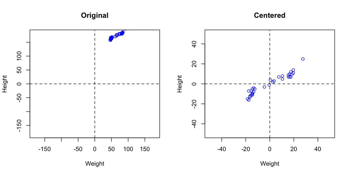
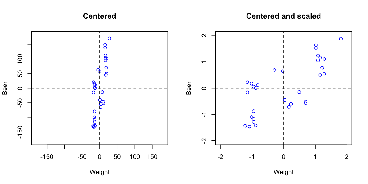
Autoscaling consists of two steps. First step is centering (or more precise mean centering) when center of data cloud in variable space is moved to an origin. Mathematically it is done by subtracting mean from the data values separately for every variable. Second step is scaling og standardization when data values are divided to standard deviation so the variables have unit variance. This autoscaling procedure (both steps) is known in statistics as standardization.

R has a built-in function for centering and scaling, scale(). The method prep.autoscale() is actually a wrapper for this function, which is mostly needed to set a proper names for the preprocessed data matrix attributes. Here are some examples how to use it (in all plots axes have the same limits to show the effect of preprocessing):

load(mdatools)
data(People)

# centering
odata = people
cdata = prep.autoscale(odata, center = T, scale = F)

plot(odata[, 'Weight'], odata[, 'Height'], 
  xlab = 'Weight', ylab = 'Height',
  col = 'blue', main = 'Original',
  xlim = c(-180, 180), ylim = c(-180, 180))
abline(h = 0, v = 0, lty = 2)

plot(cdata[, 'Weight'], cdata[, 'Height'], 
  xlab = 'Weight', ylab = 'Height',
  col = 'blue', main = 'Centered',
  xlim = c(-50, 50), ylim = c(-50, 50))
abline(h = 0, v = 0, lty = 2)

# autoscaling
adata = prep.autoscale(odata, center = T, scale = T)

par(mfrow = c(1, 2))

plot(cdata[, 'Weight'], cdata[, 'Beer'], 
  xlab = 'Weight', ylab = 'Beer',
  col = 'blue', main = 'Centered',
  xlim = c(-180, 180), ylim = c(-180, 180))
abline(h = 0, v = 0, lty = 2)

plot(adata[, 'Weight'], adata[, 'Beer'], 
  xlab = 'Weight', ylab = 'Beer',
  col = 'blue', main = 'Centered and scaled',
  xlim = c(-2, 2), ylim = c(-2, 2))
abline(h = 0, v = 0, lty = 2)

One can also use arbitrary values to center or/and scale the data, in this case use sequence or vector with these values should be provided as an argument for center or scale. Here is an example for median centering:

# median centering
mcdata = prep.autoscale(odata, center = apply(odata, 2, median))

Correction of spectral baseline

Baseline correction methods so far include Standard Normal Variate (SNV) and Multiplicative Scatter Correction (MSC).

SNV is a very simple procedure aiming first of all to remove additive and multiplicative scatter effects from Vis/NIR spectra. It is applied to every individual spectrum by subtracting its average and dividing its standard deviation from all spectral values. Here is an example:

# load UV/Vis spectra from Simdata
data(simdata)
ospectra = simdata$spectra.c

# apply SNV and show the spectra
pspectra = prep.snv(ospectra)

par(mfrow = c(2, 1))
matplot(t(ospectra), type = 'l', col = 'blue', lty = 1, main = 'Original')
matplot(t(pspectra), type = 'l', col = 'blue', lty = 1, main = 'after SNV')

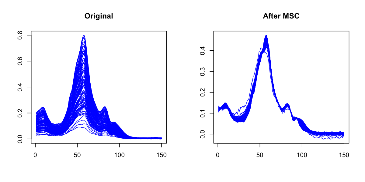
Multiplicative Scatter Correction does the same as SNV but in a different way. First it calculates a mean spectrum for the whole set (mean spectrum can be also provided as an extra argument). Then for each individual spectrum it makes a line fit for the spectral values and the mean spectrum. The coefficients of the line, intercept and slope, are used to correct the additive and multiplicative effects correspondingly.

The prep.msc() function returns a list for corrected spectra and the mean spectrum calculated for the original spectral data, so it can be reused later.

# apply MSC and and get the preprocessed spectra
res = prep.msc(ospectra)
pspectra = res$cspectra;

# show the result
par(mfrow = c(2, 1))
matplot(t(ospectra), type = 'l', col = 'blue', lty = 1, main = 'Original')
matplot(t(pspectra), type = 'l', col = 'blue', lty = 1, main = 'After MSC')

Smoothing and derivatives

Savitzky-Golay filter is used to smooth signals and calculate derivatives. The filter has three arguments: a width of the filter (width), a polynomial order (porder) and the derivative order (dorder). If the derivative order is zero (default value) then only smoothing will be performed.

# add random noise to the spectra
nspectra = ospectra + 0.025 * matrix(rnorm(length(ospectra)), dim(ospectra))

# apply SG filter for smoothing
pspectra = prep.savgol(nspectra, width = 15, porder = 1)

# apply SG filter for smoothing and take a first derivative
dpspectra = prep.savgol(nspectra, width = 15, porder = 1, dorder = 1)

# show results
par(mfrow = c(2, 2))
matplot(t(ospectra), type = 'l', col = 'blue', lty = 1, main = 'Original')
matplot(t(nspectra), type = 'l', col = 'blue', lty = 1, main = 'Noise added')
matplot(t(pspectra), type = 'l', col = 'blue', lty = 1, main = 'SG smoothing')
matplot(t(dpspectra), type = 'l', col = 'blue', lty = 1, main = '1st derivative')