Data preprocessing
The toolbox has a special object, which can be used to build a sequence of preprocessing methods and then use it either for preprocessing of original data or provide it as a preprocessing module to a model. In the latter case, every time the model is applied to a new data the data will be preprocessed first. In this chapter a brief description of the methods with several examples will be shown.
The general syntax is following. First one creates and empty preprocessing object. Then add or remove methods by using methods obj.add('name', param1, param2, ...) and obj.remove(n). Below shown a table with all currently available methods and their parameters.
| Method | Syntax | Description |
|---|---|---|
| Centering | obj.add('center', [values]) |
Center the data columns, if values are not provided, mean will be used |
| Scaling | obj.add('scale', [values]) |
Scaling data columns, if values are not provided, values will be scaled using standard deviation of the columns. |
| Normalization | obj.add('norm', type) |
Normalization of spectra either to a unit area (type is 'area') or to a unit length (type is 'length') |
| SNV | obj.add('snv') |
Standard normal variate transformation |
| MSC | obj.add('msc', [mean]) |
Multiplicative scatter correction, the optional argument mean is a vector with mean spectrum values (will be calculated from the data values if not provided) |
| ALS baseline correction | obj.add('alsbasecorr', s, p) |
Baseline correction with Asymmetric Least Squares. The paramater sis a smoothness (default is 100000), and pis a penalty (default is 0.1). |
| Savitzky-Golay transformation | obj.add('savgol', d, w, p) |
Savitzky-Golay transformation, dis a derivative (use 0 for no derivative), wis a size of the filter (3, 5, 7, ...) and p is a polynomial degree. |
| Whitening | obj.add('whitening') |
Whitening transformation to make observations uncorrelated and with unit variance (useful for Independent Component Analysis). |
| Reflectance to absorbance | obj.add('ref2abs') |
Transforms reflectance spectra to absorbance spectra with log(1/R) transformation. |
Let us show how all these work starting with two simple preprocessing methods, centering and standardization, and later show details for several other.
Autoscaling
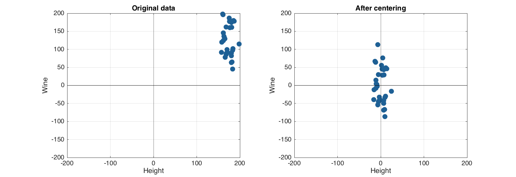
Autoscaling consists of two steps. First step is centering (or, more precise, mean centering) when center of a data cloud in variable space is moved to an origin. Mathematically it is done by subtracting mean from the data values separately for every variable. Second step is standardization (or scaling) when data values are divided to standard deviation so the variables have unit variance.
Here are some examples how apply these two operations in mdatools (in all plots axes have the same limits to show the effect of preprocessing). We start with creating object with centering.
load(people)

% we will use variables Wine and Height
data = people(:, {'Wine', 'Height'});

% create a preprocessing object only for centering
p = prep();
p.add('center');

% show information about the object
show(p);
Preprocessing ("prep") object
methods included: 1
1. center (mean centering)

Use "obj.add(name, properties)" to add a new method.
Use "obj.remove(n)" to remove a method from the list.

See "help prep" for list of available methods.
Method show()displays the list of added preprocessing methods, their order as well as some help information. Now we can apply the preprocessing methods of the created object to the data. In order to compare the original and preprocessed data we create a copy for the dataset and use the same scale (–200, 200) for axes on both plots.
% create a copy of dataset and apply preprocessing
pdata1 = copy(data);
p.apply(pdata1);


% show the results
lim = 200;
figure

subplot 121
scatter(data)
title('Original data')
grid on
axis([-lim lim -lim lim])

subplot 122
scatter(pdata1)
title('After centering')
grid on
axis([-lim lim -lim lim])
Now let us create a reprocessing object for autoscaling by adding both centering and scaling (standardization) to the object.
p = prep();
p.add('center');
p.add('scale');

show(p);
Preprocessing ("prep") object
methods included: 2
1. center (mean centering)
2. scale (standardization)

Use "obj.add(name, properties)" to add a new method.
Use "obj.remove(n)" to remove a method from the list.

See "help prep" for list of available methods.
And apply the methods to the original data.
pdata2 = copy(data);
p.apply(pdata2);

figure

subplot 121
scatter(pdata1)
title('After centering')
grid on
axis([-100 100 -100 100])

subplot 122
scatter(pdata2)
title('After autoscaling')
grid on
axis([-2 2 -2 2])

One can also use arbitrary values to center or/and scale the data, in this case use sequence or vector with these values should be provided as an argument for center or scale. Here is an example for median centering:
p = prep();
p.add('center', median(data));
Any method can be removed from the sequence by using its number.
p = prep();
p.add('center');
p.add('scale');

show(p);
Preprocessing ("prep") object
methods included: 2
1. center (mean centering)
2. scale (standardization)

Use "obj.add(name, properties)" to add a new method.
Use "obj.remove(n)" to remove a method from the list.

See "help prep" for list of available methods.
p.remove(1);

show(p);
Preprocessing ("prep") object
methods included: 1
1. scale (standardization)

Use "obj.add(name, properties)" to add a new method.
Use "obj.remove(n)" to remove a method from the list.

See "help prep" for list of available methods.
A preprocessing object can also be applied to an ordinary MATLAB matrix (not dataset), in this case one just has to specify a variable to get the preprocessing results:
x = randn(5, 2) * 2 + 10;
disp(x)
    6.1951    6.6305
   14.7485   10.8263
    9.5333   11.0035
   10.8078   10.1661
   12.3849   10.3156
p = prep();
p.add('center');
p.add('scale');

y = p.apply(x);
disp(y)
   -1.4196   -1.7553
    1.2556    0.5769
   -0.3755    0.6754
    0.0231    0.2100
    0.5164    0.2930
Parameters of preprocessing
Some of the methods (e.g. scaling, centering, MSC transformation) have one or several parameters, either provided by a user, or calculated automatically when apply a particular method for the first time. After this, the method "remembers" the calculated values and if we apply it again to another data it will use the saved values instead of calculating the new ones. Here is an example of this behavior for centering.
First we split People data for males and females and take only first five variables:
load('people')

m = people(people(:, 'Sex') == -1, 1:5);
f = people(people(:, 'Sex') ==  1, 1:5);
Then we create a preprocessing object for centering and apply it to females:
p = prep();
p.add('center');

fp = copy(f);
p.apply(fp);

show(mean(f))
show(mean(fp))
                     Variables
      Height  Weight  Hairleng  Shoesize   Age
     ------- ------- --------- --------- -----
Mean     164    50.8     0.875      36.4  31.1


                     Variables
      Height  Weight  Hairleng  Shoesize  Age
     ------- ------- --------- --------- ----
Mean       0       0         0         0    0
As one can notice, the data is perfectly centered. However, if we use the same preprocessing object for centering the male data, we will get the following:
mp = copy(m);
p.apply(mp);

show(mean(m))
show(mean(mp))
                     Variables
      Height  Weight  Hairleng  Shoesize   Age
     ------- ------- --------- --------- -----
Mean     182    78.2    -0.875      43.4  37.8


                     Variables
      Height  Weight  Hairleng  Shoesize   Age
     ------- ------- --------- --------- -----
Mean    17.4    27.4     -1.75      7.06  6.62
We can see that the data values for the males were not centered correctly, because when we applied the preprocessing first time, the preprocessing object has calculated mean values for female objects and saved them. So when we applied the object to the male data, the saved values were used, which are of course different from the mean values of the male persons in the dataset.
If you want to "reset" all settings without creating a new preprocessing object manually just create a copy of the existent one:
p2 = copy(p);
mp = copy(m);
p2.apply(mp)

show(mean(m))
show(mean(mp))
                     Variables
      Height  Weight  Hairleng  Shoesize   Age
     ------- ------- --------- --------- -----
Mean     182    78.2    -0.875      43.4  37.8


                     Variables
      Height  Weight  Hairleng  Shoesize  Age
     ------- ------- --------- --------- ----
Mean       0       0         0         0    0
Correction of spectral baseline
Baseline correction methods so far include Standard Normal Variate (SNV), Multiplicative Scatter Correction (MSC) and baseline correction with Asymmetric Least Squares.
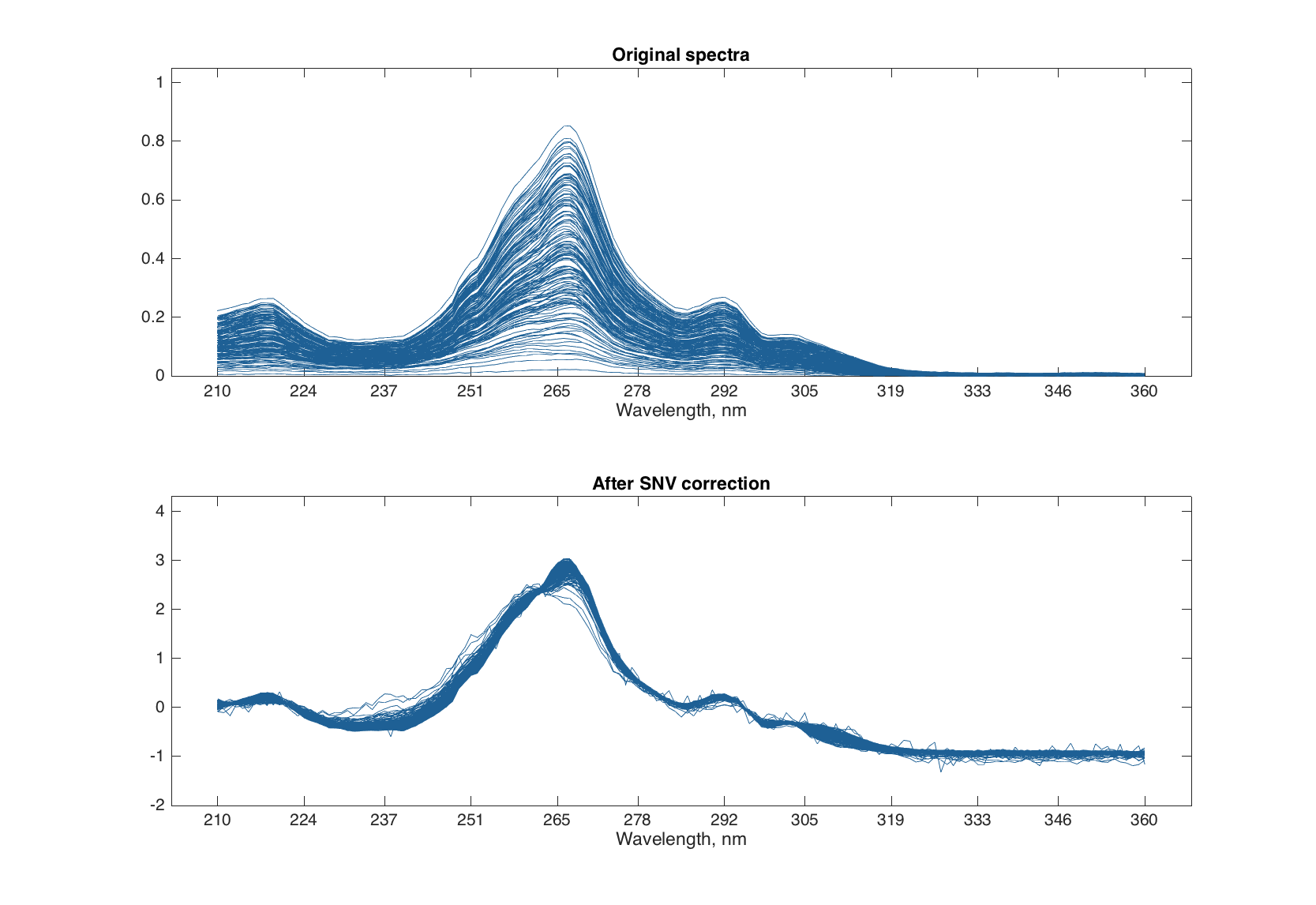
SNV is a very simple procedure aiming first of all to remove additive and multiplicative scatter effects from Vis/NIR spectra. It is applied to every individual spectrum by subtracting its average and dividing its standard deviation from all spectral values. Here is an example:
% load UV/Vis spectra from Simdata
load('simdata')

% create a preprocessing object
p = prep();
p.add('snv')

% create a copy of spectra and apply preprocessing
pspectra = copy(spectra);
p.apply(pspectra)

% show the results
figure

subplot 211
plot(spectra)
title('Original spectra')

subplot 212
plot(pspectra)
title('After SNV correction')
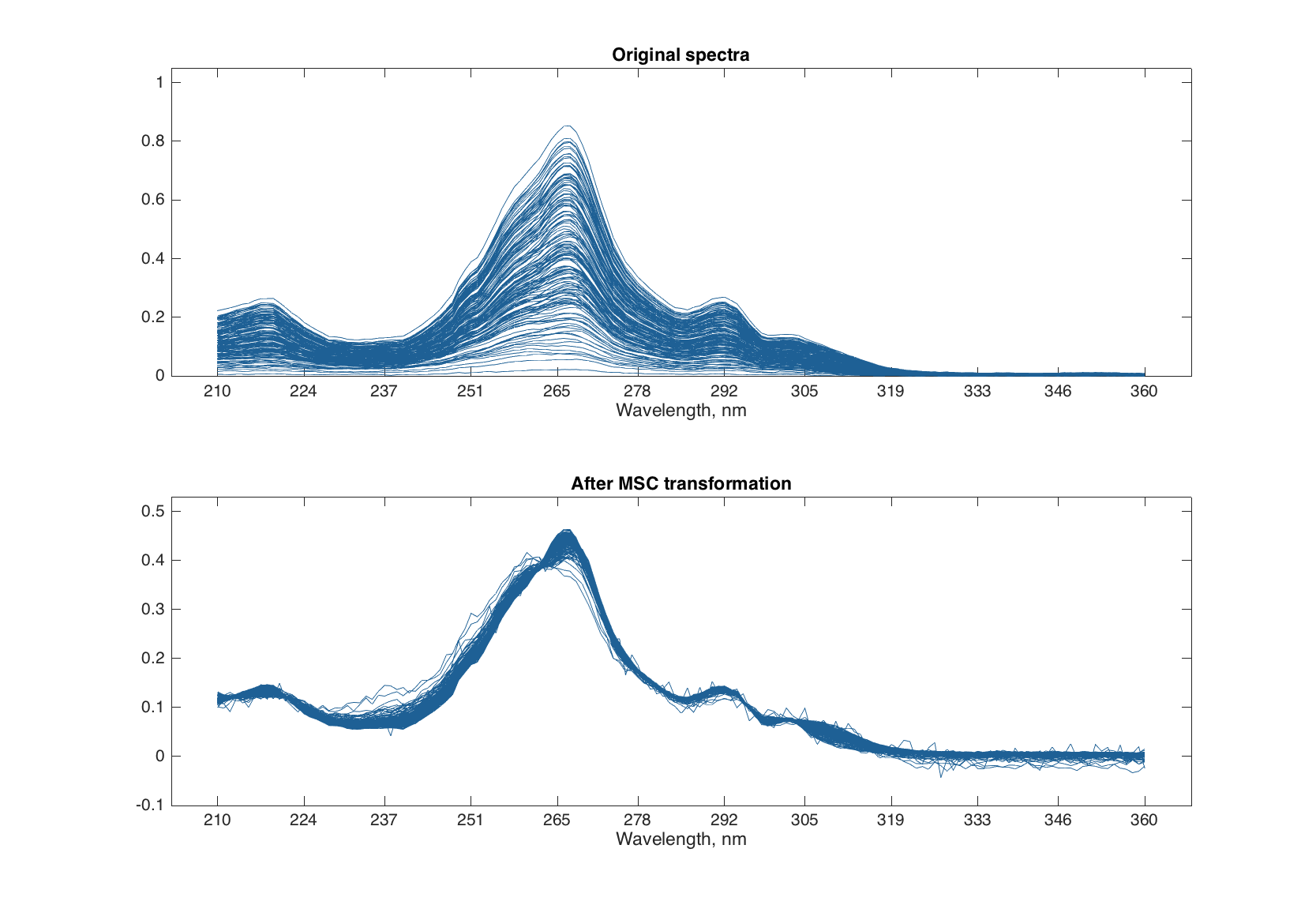
Multiplicative Scatter Correction does the same as SNV but in a different way. First it calculates a mean spectrum for the whole set (mean spectrum can be also provided as an extra argument). Then, for each individual spectrum, it makes a line fit for the spectral values and the mean spectrum. The coefficients of the line, intercept and slope, are used to correct the additive and multiplicative effects correspondingly.
% create a preprocessing object
p = prep();
p.add('msc');

% create a copy of spectra and apply preprocessing
pspectra = copy(spectra);
p.apply(pspectra);

% show the result
figure

subplot 211
plot(spectra)
title('Original spectra')

subplot 212
plot(pspectra)
title('After MSC transformation')
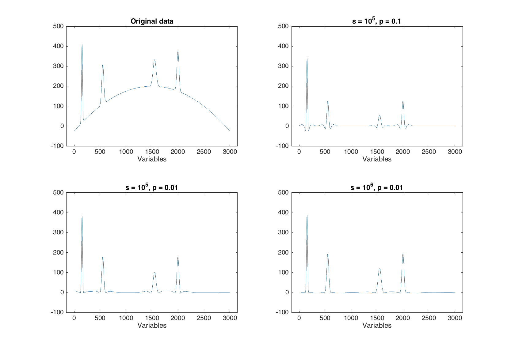
The ALS baseline correction is very useful for removing baseline issues in spectroscopic data with relatively narrow peaks, such as Raman, IR and similar. The method has two parameters — smoothness (s, default 100000) and penalty (p, default 0.1). In the code below we generate a signal with four narrow peaks and baseline shape as a quadratic polynomial and use the ALS approach to "correct" the baseline.
% function for normal distribution PDF
npdf = @(x, m, s)(1/sqrt(2 * pi * s^2) * exp(-(x - m).^2/(2 * s^2)));

% generate signal
x = 1:3000;
y = -((x - 1500) / 100).^2 + 200;
y = y + npdf(x, 150, 10) * 10000;
y = y + npdf(x, 550, 20) * 10000;
y = y + npdf(x, 1550, 30) * 10000;
y = y + npdf(x, 2000, 20) * 10000;
y = mdadata(y);

% create three preprocessing objects
p1 = prep(); p1.add('alsbasecorr', 100000, 0.1);
p2 = prep(); p2.add('alsbasecorr', 100000, 0.01);
p3 = prep(); p3.add('alsbasecorr', 1000000, 0.01);

% apply preprocessing to copies of the signal
py1 = copy(y);
p1.apply(py1);
py2 = copy(y);
p2.apply(py2);
py3 = copy(y);
p3.apply(py3);

% show results
figure

subplot 221
plot(y)
ylim([-100 500])
title('Original data')

subplot 222
plot(py1)
ylim([-100 500])

subplot 223
plot(py2)
ylim([-100 500])

subplot 224
plot(py3)
ylim([-100 500])
Smoothing and derivatives
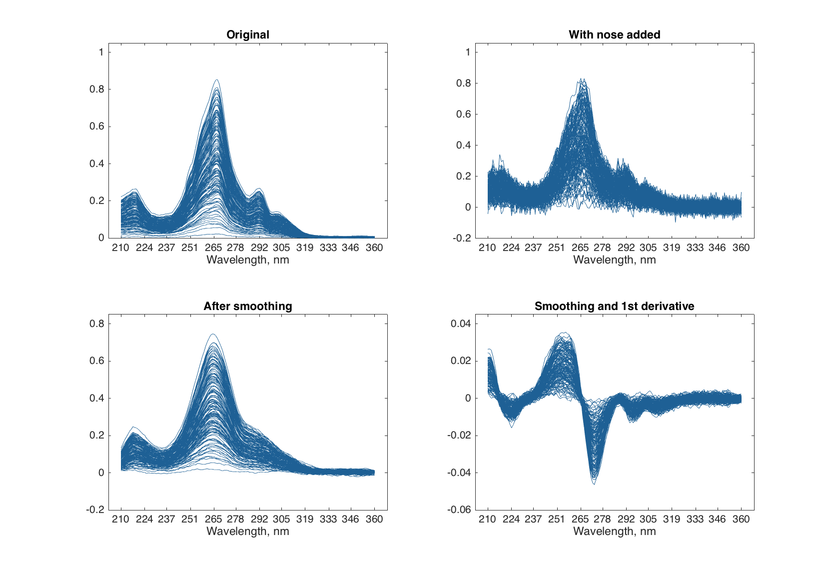
Savitzky-Golay filter is used to smooth signals and calculate derivatives. The filter has three arguments: a derivative order (d), a width of the filter (w), and a polynomial degree (p). If the derivative order is zero (default value) then only smoothing will be performed. Below are some examples of using this filter for the Simdata spectra with added random noise.
load('simdata')

% add random noise to the spectra
nspectra = spectra + 0.025 * randn(size(spectra));

% create two objects for preprocessing
p1 = prep();
p1.add('savgol', 0, 15, 1);

p2 = prep();
p2.add('savgol', 1, 15, 1);

% apply the preprocessing
sspectra = copy(nspectra);
p1.apply(sspectra);

dspectra = copy(nspectra);
p2.apply(dspectra);

% show results
figure

subplot 221
plot(spectra)
title('Original')
subplot 222
plot(npectra)
title('With nose added')
subplot 223
plot(sspectra)
title('After smoothing')
subplot 224
plot(dspectra)
title('Smoothing and 1st derivative')
Mathematical functions
Any math function, such as for example power or logarithm can also become a part of a preprocessing object. The general syntax is following:
obj.add('math', @fun, param1, param2, ...)
Here @fun is a function handle and all parameters are optional. Here is a simple example:
p = prep();
p.add('math', @log);
p.add('math', @power, 1.5);

show(p)
Preprocessing ("prep") object
methods included: 2
1. math (Mathematical function: log)
2. math (Mathematical function: power)

Use "obj.add(name, properties)" to add a new method.
Use "obj.remove(n)" to remove a method from the list.

See "help prep" for list of available methods.
x = 1:5

y = p.apply(x);
disp(y)
0 0.5771 1.1515 1.6322 2.0418